Sunday 6 March 2016

Triaging with `pidstat`

This post will detail a few example uses of the `pidstat` tool while digging into performance of a Graphite instance.

Without taking any measurements, reading up a bit on Graphite's architecture can help shed some light on what is going on under the hood.  At the very minimum, we know the following about the application:
  • Receives metrics over a network interface
  • Stores metrics to disk
  • Generates graphs in response to requests over a network interface
The above functionality allows for the possibility of the following bottlenecks:
  • I/O-bound from disk I/O
  • I/O bound from network I/O
  • CPU-bound from I/O co-ordination
I'm expecting the system to be CPU-bound as previous tuning iteration with this system was in response to saturation of the CPU. This has led to the current state where there is a `carbon-cache` instance running for each core available to the system as well as a single carbon-relay running to load-balance traffic to each carbon-cache process.  Given this knowledge, a good place to start poking around would be the `carbon-relay` instance.

I'll begin with examining CPU utilization of the process.

pidstat -u -p 25430 1
Linux 3.13.0-43-generic (stats.tunnelbear.com)  16-02-10        _x86_64_        (4 CPU)

03:24:05 AM   UID       PID    %usr %system  %guest    %CPU   CPU  Command
03:24:06 AM   999     25430   57.00    2.00    0.00   59.00     1  carbon-relay.py
03:24:07 AM   999     25430   49.00    2.00    0.00   51.00     2  carbon-relay.py
03:24:08 AM   999     25430   71.00    2.00    0.00   73.00     2  carbon-relay.py
03:24:09 AM   999     25430   50.00    2.00    0.00   52.00     0  carbon-relay.py
03:24:10 AM   999     25430   26.00    2.00    0.00   28.00     2  carbon-relay.py
03:24:11 AM   999     25430   38.00    1.00    0.00   39.00     2  carbon-relay.py
03:24:12 AM   999     25430   38.00    1.00    0.00   39.00     2  carbon-relay.py
03:24:13 AM   999     25430   44.00    2.00    0.00   46.00     2  carbon-relay.py
03:24:14 AM   999     25430   30.00    2.00    0.00   32.00     2  carbon-relay.py
03:24:15 AM   999     25430   35.00    0.00    0.00   35.00     2  carbon-relay.py
03:24:16 AM   999     25430   68.00    2.00    0.00   70.00     2  carbon-relay.py
03:24:17 AM   999     25430   76.00    1.00    0.00   77.00     2  carbon-relay.py
03:24:18 AM   999     25430   70.00    3.00    0.00   73.00     2  carbon-relay.py
03:24:19 AM   999     25430   41.00    4.00    0.00   45.00     2  carbon-relay.py
03:24:20 AM   999     25430   36.00    2.00    0.00   38.00     2  carbon-relay.py
03:24:21 AM   999     25430   32.00    2.00    0.00   34.00     2  carbon-relay.py
03:24:22 AM   999     25430   28.00    1.00    0.00   29.00     2  carbon-relay.py
03:24:23 AM   999     25430   38.00    2.00    0.00   40.00     2  carbon-relay.py
03:24:24 AM   999     25430   53.00    2.00    0.00   55.00     0  carbon-relay.py
03:24:25 AM   999     25430   71.00    1.00    0.00   72.00     2  carbon-relay.py
03:24:26 AM   999     25430   78.00    3.00    0.00   81.00     2  carbon-relay.py
^C
Average:      999     25430   49.00    1.86    0.00   50.86     -  carbon-relay.py
Here, I've used the `pidstat` utility while specifying the PID of the carbon-relay instance, setting the CPU statistics flag and requesting updates every 1 second.

Some interesting observations are:
  • The `carbon-relay` instance is typically serviced by CPU 2 but it is not strictly pinned to it.
  • The average total percentage of CPU time used by the `carbon-relay` instance is around 50%.
  • Around 96% of the time the `carbon-relay` instance is executing at the user level leaving a small percentage of associated work within kernel space.
How does this compare to a `carbon-cache` process?

pidstat -u -p 24569 1                                                                                                                                                           
Linux 3.13.0-43-generic (stats.tunnelbear.com)  16-02-10        _x86_64_        (4 CPU)

03:30:35 AM   UID       PID    %usr %system  %guest    %CPU   CPU  Command
03:30:36 AM   999     24569   16.00    8.00    0.00   24.00     1  carbon-cache.py
03:30:37 AM   999     24569   16.00    6.00    0.00   22.00     2  carbon-cache.py
03:30:38 AM   999     24569   10.00    4.00    0.00   14.00     2  carbon-cache.py
03:30:39 AM   999     24569    7.00    2.00    0.00    9.00     2  carbon-cache.py
03:30:40 AM   999     24569    6.00    3.00    0.00    9.00     2  carbon-cache.py
03:30:41 AM   999     24569    8.00    4.00    0.00   12.00     2  carbon-cache.py
03:30:42 AM   999     24569    9.00    2.00    0.00   11.00     3  carbon-cache.py
03:30:43 AM   999     24569   18.00   10.00    0.00   28.00     0  carbon-cache.py
03:30:44 AM   999     24569   12.00    5.00    0.00   17.00     3  carbon-cache.py
03:30:45 AM   999     24569    8.00    3.00    0.00   11.00     2  carbon-cache.py
03:30:46 AM   999     24569   17.00    6.00    0.00   23.00     1  carbon-cache.py
03:30:47 AM   999     24569    4.00    3.00    0.00    7.00     3  carbon-cache.py
03:30:48 AM   999     24569    5.00    0.00    0.00    5.00     1  carbon-cache.py
03:30:49 AM   999     24569   11.00    4.00    0.00   15.00     1  carbon-cache.py
03:30:50 AM   999     24569   17.00    8.00    0.00   25.00     1  carbon-cache.py
03:30:51 AM   999     24569   10.00    8.00    0.00   18.00     1  carbon-cache.py
03:30:52 AM   999     24569    8.00    3.00    0.00   11.00     1  carbon-cache.py
03:30:53 AM   999     24569    5.00    3.00    0.00    8.00     0  carbon-cache.py
03:30:54 AM   999     24569   15.00    7.00    0.00   22.00     1  carbon-cache.py
03:30:55 AM   999     24569   11.00    6.00    0.00   17.00     1  carbon-cache.py
03:30:56 AM   999     24569    4.00    1.00    0.00    5.00     0  carbon-cache.py
03:30:57 AM   999     24569   12.00    8.00    0.00   20.00     0  carbon-cache.py
03:30:58 AM   999     24569   15.00    5.00    0.00   20.00     0  carbon-cache.py
03:30:59 AM   999     24569   19.00   10.00    0.00   29.00     0  carbon-cache.py
03:31:00 AM   999     24569    9.90    5.94    0.00   15.84     0  carbon-cache.py
03:31:01 AM   999     24569   12.00    6.00    0.00   18.00     1  carbon-cache.py
03:31:02 AM   999     24569    9.00    7.00    0.00   16.00     0  carbon-cache.py
03:31:03 AM   999     24569    3.00    1.00    0.00    4.00     2  carbon-cache.py
03:31:04 AM   999     24569   14.00    4.00    0.00   18.00     1  carbon-cache.py
03:31:05 AM   999     24569   10.00    3.00    0.00   13.00     1  carbon-cache.py
03:31:06 AM   999     24569   18.00    9.00    0.00   27.00     1  carbon-cache.py
^C
Average:      999     24569   10.93    5.00    0.00   15.93     -  carbon-cache.py
Using a similar `pidstat` call while targeting the PID of a carbon-cache instance yields the following comparative observations:
  • The `carbon-relay` instance taxes processing resources more than the previously examined `carbon-cache` instance.
  • The `carbon-relay` instance executes mainly in user space while it's counterpart operates at a 2:1 ratio between user and kernel space (most likely due to disk I/O).
`pidstat` can also report on context switching activity.  The following snippets are the summary outputs from a pair of `pidstat` calls targeting the relay and cache instances:

01:22:44 AM   UID       PID   cswch/s nvcswch/s  Command
Average:      999     12028     66.94      2.47  carbon-cache.py
Average:      999     12043     71.11    164.32  carbon-relay.py
The average number of voluntary context switches per second are similar while average non-voluntary context switches are much higher for the `carbon-relay` instance.

Voluntary context switches occur when a task blocks because it requires a resource that is unavailable.  Comparing these two processes in terms of voluntary context switches, it seems as if the values are quite close.  Other unrelated processes on the system have values closer to zero while also having CPU time quite low.  Although these processes are functionally related due to them being apart of the same application, they have completely different CPU workloads.  Their similarity in voluntary context switch rate could use some more investigation.

Non-voluntary context switches occur when a task's time slice runs to completion and it is forced away from processing in favour of the next task in line.  Looking at the averages above, the non-voluntary context switches per second that the `carbon-relay` instance is experiencing sticks out and could use some further investigation.

Digging deeper past this initial triage can be done with other tools such as SystemTap or perf to uncover the code paths contributing to this performance.

Sunday 21 February 2016

Generating Debug Symbols for the Linux Kernel

While working with SystemTap on an Ubuntu 14.04 installation, I was met with the following error when trying to probe a syscall:

Systemtap translator/driver (version 2.3/0.158, Debian version 2.3-1ubuntu1.1 (trusty))
Copyright (C) 2005-2013 Red Hat, Inc. and others
This is free software; see the source for copying conditions.
enabled features: AVAHI LIBSQLITE3 NSS TR1_UNORDERED_MAP NLS
Created temporary directory "/tmp/stapJqcNkt"
Session arch: x86_64 release: 3.13.0-43-generic
Kernel symbol table /lib/modules/3.13.0-43-generic/build/System.map unavailable, (No such file or directory)
Searched for library macro files: "/usr/share/systemtap/tapset/linux/*.stpm", found: 2, processed: 2
Searched for library macro files: "/usr/share/systemtap/tapset/*.stpm", found: 1, processed: 1
Searched: "/usr/share/systemtap/tapset/linux/x86_64/*.stp", found: 3, processed: 3
Searched: "/usr/share/systemtap/tapset/linux/*.stp", found: 67, processed: 67
Searched: "/usr/share/systemtap/tapset/x86_64/*.stp", found: 1, processed: 1
Searched: "/usr/share/systemtap/tapset/*.stp", found: 21, processed: 21
Pass 1: parsed user script and 95 library script(s) using 85852virt/27404res/2536shr/25488data kb, in 120usr/40sys/161real ms.
Attempting to extract kernel debuginfo build ID from /lib/modules/3.13.0-43-generic/build/vmlinux.id
Attempting to extract kernel debuginfo build ID from /sys/kernel/notes
semantic error: while resolving probe point: identifier 'syscall' at open.stp:1:7
        source: probe syscall.open
                      ^

semantic error: no match
Pass 2: analyzed script: 0 probe(s), 0 function(s), 0 embed(s), 0 global(s) using 86364virt/28296res/2792shr/26000data kb, in 40usr/360sys/1130real ms.
Pass 2: analysis failed.  [man error::pass2]
Tip: /usr/share/doc/systemtap/README.Debian should help you get started.
Running rm -rf /tmp/stapJqcNkt
Spawn waitpid result (0x0): 0
Removed temporary directory "/tmp/stapJqcNkt"
To get around this, I ended up having to generate the debug symbols for the installed Linux kernel so that SystemTap could consume them while setting up the probe.  The rest of this post describes the steps that were taken to complete this task.

Build preparation

Apt provides the `build-dep` operation which pulls in all of the build dependencies that would be needed to build the specified source package.  In this case, the following command did the trick:
sudo apt-get build-dep --no-install-recommends linux-image-$(uname -r)
Pulling down the kernel source code can be accomplished via Apt as the `source` operation makes this possible:
apt-get source linux-image-$(uname -r)
This had unexpected results however as the currently running kernel reported by `uname -r` that was requested was not delivered due to a newer version being available:
Reading package lists... Done
Building dependency tree
Reading state information... Done
Picking 'linux' as source package instead of 'linux-image-3.13.0-43-generic'
NOTICE: 'linux' packaging is maintained in the 'Git' version control system at:
http://kernel.ubuntu.com/git-repos/ubuntu/ubuntu-trusty.git
Need to get 126 MB of source archives.
Get:1 http://mirrors.digitalocean.com/ubuntu/ trusty-updates/main linux 3.13.0-77.121 (dsc) [8,019 B]
Get:2 http://mirrors.digitalocean.com/ubuntu/ trusty-updates/main linux 3.13.0-77.121 (tar) [116 MB]
Get:3 http://mirrors.digitalocean.com/ubuntu/ trusty-updates/main linux 3.13.0-77.121 (diff) [9,076 kB]
Fetched 126 MB in 5s (21.4 MB/s)
I ended up having to clone the kernel version I wanted via git:
git clone git://kernel.ubuntu.com/ubuntu/ubuntu-<release>.git
git checkout -b temp Ubuntu-<kernel_version>

Build the kernel

Once the kernel source code was accessible and all build dependencies were in place, I was able to build the kernel alongside the desired debug symbols:
fakeroot debian/rules clean
AUTOBUILD=1 fakeroot debian/rules binary-generic skipdbg=false
The above commands essentially invoke the build script that is bundled with the kernel source code.  Leveraging `fakeroot` allows for the resulting build to contain files or directories that have root permissions assigned to them without having to run the overall build script as the root user.  Also note that the `skipdbg=false` flag is present which accomplishes generating a kernel that includes the debug symbols necessary for SystemTap to function.

Install the kernel debug symbols

The final step was to install the newly built kernel with accompanying debug symbols via `dpkg`:
dpkg -i ../linux-image-3.13.0-43-generic-dbgsym_3.13.0-43.121_amd64.ddeb

References

https://wiki.ubuntu.com/Kernel/Systemtap
https://wiki.ubuntu.com/Kernel/BuildYourOwnKernel
https://wiki.ubuntu.com/KernelTeam/KernelMaintenance
https://wiki.ubuntu.com/Kernel/SourceCode

Sunday 14 February 2016

Linux Load Average

For Linux systems, the load average reported via commands such as `uptime` is "a measure of the average number of processes that are either in a runnable or uninterruptable state".

To be more concrete, the following scenarios all contribute to the load average metric:
  • A unit of work is on-CPU and being executed
  • A unit of work is off-CPU in the schedule queue waiting for it's turn to be on-CPU
  • A unit of work is waiting for an I/O resource to become available (disk/network)
Therefore, it is useful to keep in mind that load is not strictly a measure of CPU "busyness" since for Linux systems I/O plays a part in the value that is calculated.

Wednesday 3 February 2016

Advanced IPTables Matching

Here are a few examples of advanced iptables matching rules.  Note that lines with multiple match rules have the heavier rules ordered last.  This subjects a subset of all traffic to the heavy processing required for operations such as string matching as least costly match rules shield all traffic from the costly match rules.

Matching TLS traffic to specific domains

iptables -I FORWARD -p tcp --dport 443 ! -f -m state --state ESTABLISHED -m u32 --u32 "0>>22&0x3C@ 12>>26&0x3C@ 0>>24 & 0xFF=0x16 && 0>>22&0x3C@ 12>>26&0x3C@ 2>>24 & 0xFF=0x01" --algo bm -j LOG --log-prefix "TLS Client Hello: "
Match on TCP traffic to port 443 that has already been established and is not a fragment
-p tcp --dport 443 ! -f -m state --state ESTABLISHED
Use the u32 module for byte matching
-m u32 --u32
Fast forward past the IP header
0>>22&0x3C@
Fast forward past the TCP header
12>>26&0x3C@
Match when the first byte of the TCP payload is 0x16 (or decimal 22 signifying a TLS record)
0>>24 & 0xFF=0x16
Match when the above conditions are true as well as having the 6th byte of the TCP payload equalling 0x01 (signifying a ClientHello)
0>>22&0x3C@ 12>>26&0x3C@ 2>>24 & 0xFF=0x01

If a specific domain is needed, iptables can  scan the matched TLS ClientHelllo for the string 'domain'
-m string --string "domain" --algo bm

Forcing AAAA record DNS resolution for specific domains

iptables -I INPUT -p udp --dport 53 -m string --hex-string '|<domain name encoded as hex string>0001|' --algo bm -j DROP

Match on DNS traffic (UDP/53)
-p udp --dport 53

Match on the target domain string followed by a DNS Query Type 0x01 (A Record):
-m string --hex-string '|<domain name encoded as hex string>0001|' --algo bm

Drop these requests:
-j DROP

Modern browsers should be sending both A and AAAA DNS queries.  By dropping the A queries, the AAAA responses would be the only responses allowed for the target domain thus forcing IPv6 connectivity.

Thursday 18 October 2012

Distributed ANN

The following report describes the logic behind a distributed artificial neural network that I created for the purpose of testing the integration between Contiki OS and ns-3.  The accompanying Contiki code is linked as well.  Note that the integration component is forecasted for release into the ns-3 community by the end of the year.  If there is interest in the integration component, please let me know and I can make it available outside of the ns-3 channels.  The ns-3 code can be found here for anyone to use or fork.


Documentation
Contiki Code

Tuesday 28 August 2012

Contiki OS

Preface

I recently had the opportunity to work on an integration between the Contiki OS and the ns-3 network simulator.  I found that documentation was sparse on the Contiki side and ended up having to dig through the source code to understand its operation.  The following post encompasses my findings which were also submitted as a degree requirement for the MEng. Computer Networks program at Ryerson University.

Please excuse any out of context references as this was pulled from a paper that was not solely focused on Contiki.

Contiki OS Scheduler


The Contiki Operating System came to existence as an extension of the uIP network stack, which was developed out of the Swedish Institute of Computer Science.  Its design allows for features such as multi-tasking, multiple threaded processes, remote GUI and a fully functioning customizable network stack – the RIME stack – along with the original uIP stack [3].  Being extremely lightweight, the operating system only requires around 100 KB of memory for core operations, which makes it suitable for memory-constrained devices such as microcontrollers.  Applications for Contiki include streetlights, home and factory automation devices, security devices and various industry-specific monitoring devices. 

Looking under the hood, the remainder of this section examines the scheduler at the core of the Contiki OS.  
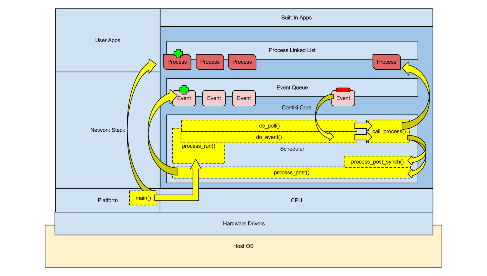
The following graphic displays the flow of control within the kernel.


Looking at the figure above, all processing begins with the main() function within the Platform code visually depicted on the bottom left of the diagram.  The main() function, usually defined within the platform-specific code (i.e. contiki/platform/ns3) starts a set of concurrent processes using the PROCINIT macro:

PROCINIT(&etimer_process, &tapdev_process, &tcpip_process, &serial_line_process);

The set of listed processes can be user applications, device drivers, network stacks or other optional core functionality depending on the overall function of the Contiki node. For example, the minimal-net platform requires a tap device connecting into the underlying host OS and therefore defines the &tapdev_process in its set of processes to start.  Once all processes are started, control shifts to the scheduler.  The driving function, process_run(), is usually called within a while loop from the main() function.  process_run() then schedules a series of functions that do the following:
  • Checks a poll flag typically set by device driver processes, event timer processes, and any process utilizing IPC.  If set, the process' poll handler function (the function defined to respond to the PROCESS_EVENT_POLL event) will be called immediately.
  • Adds events to the event queue.
  • Removes events from the event queue.
  • Processes the functionality of the removed events by giving control to the process specified in the event which resides in the process list. 
The default scheduling algorithm pulls events from the front of the queue while ensuring that polling is done in between processing events.  An event can either schedule subsequent events at the back of the event queue via the process_post() function or can immediately call a process to skip queuing with the process_post_synch() function.  Polling results in a device, event timer, or IPC-enabled process immediately running its poll handler function which can make use of the process_post() and process_post_synch() functions to schedule further events or run other functions.

When data from the application layer is generated, an event is scheduled to invoke the configured NET/MAC stack so that it can read from the application layer.  When the event reaches the front of the event queue, the network stack will operate on the layer 7 data in memory and then pass its pointer down further to the configured hardware driver by scheduling either targeted events (i.e. TCP_POLL used to indicate data is ready for the network layer from the transport layer) or general events (i.e. PROCESS_EVENT_POLL).  When this event is at the front of the event queue the correct process can be called using an event addressing mechanism that ensures that the correct member function can be called based on the selected event name.

Data on its way in from the hardware relies on poll flags to interrupt sequential event queue processing.  When data arrives, it is written to memory and the receiving device driver process sets a poll flag.  Between subsequent events, the poll flag belonging to each process is checked.  If a flag is found to be set, the process' poll handler function is invoked which is defined by the PROCESS_POLLHANDLER macro.  Therefore, in between subsequent scheduled events there is always an opportunity for some network I/O to occur.  A device driver can include both input and output in its poll handler.  

For example, data can originate from the application layer and be written to the single memory buffer reserved for network I/O.  An event can be scheduled at the back of the event queue to send this data out via the hardware.  Before this event reaches the front of the queue, incoming data from the hardware can signal the device driver to set the poll flag concurrent to event queue processing.  After the next event is processed, the poll flag is checked for all processes revealing that the network device has some work to do.  The poll handler function is called that writes the data that has been prepared by the APP/NET/MAC layers before the scheduled event for this write action has reached the front of the event queue.  Additionally, the poll handler reads the incoming data from the hardware buffer into the newly freed data buffer for the APP/NET/MAC layers to operate on in the upwards network stack direction.  The poll handler finishes and control is given back to event queue processing.

Contiki OS Network Stack Architecture


Choosing a MAC protocol is performed by mapping function pointers to appropriate functions.  The network stack is defined in the platform/…/contiki-conf.h configuration header file, which takes a modular approach to the network layer, radio duty cycle, MAC layer, radio driver, and framing.  Each configurable element of the network stack is represented by a structure as shown in the code snippet below:

extern const struct network_driver NETSTACK_NETWORK;
extern const struct rdc_driver NETSTACK_RDC;
extern const struct mac_driver NETSTACK_MAC;
extern const struct radio_driver NETSTACK_RADIO;
extern const struct framer NETSTACK_FRAMER;

Each structure is originally defined in its own header file where a list of required functions accompany the structure. For example, in core/net/mac/mac.h there are six function pointers defined.

struct mac_driver {
char *name;
/** Initialize the MAC driver */
void (* init)(void);
/** Send a packet from the Rime buffer */
void (* send)(mac_callback_t sent_callback, void *ptr);
/** Callback for getting notified of incoming packet. */
void (* input)(void);
/** Turn the MAC layer on. */
int (* on)(void);
/** Turn the MAC layer off. */
int (* off)(int keep_radio_on);
/** Returns the channel check interval, expressed in clock_time_t ticks. */
unsigned short (* channel_check_interval)(void);
};

Any MAC protocol chosen for compilation into the Contiki executable must provide the required functions and also modify the struct defined in netstack.h to apply the function pointers to the defined functions. An example of this is shown below pulled from core/net/mac/csma.c:

const struct mac_driver csma_driver = {
"CSMA",
init,
send_packet,
input_packet,
on,
off,
channel_check_interval,
};


The diagram above displays the flow of control within the Contiki OS during network input.  Data originates packaged with all layer headers via the hardware driver process.  In this case, the socketradio.c/h files specify how to pull information from the underlying OS IPC socket. The raw data is copied from the socket to the packetbuf memory buffer, which is typically reserved for MAC layer processing of data. The faint green arrow displays this movement of data from the socket to the memory buffer.  Control then shifts from the device driver process into the OS network stack.  The network stack is a series of preconfigured (during compilation) function calls that chain into each other up and down the stack.  For sicslowpan/sicslowmac, the network stack is composed of the sicslowpan driver (network layer), the nullmac driver (MAC layer), the sicslowmac driver (Radio Duty Cycle), the framer802154 driver (Framer), and a variable radio driver that was chosen to be the socketradio device driver in this case to socket communication with ns-3.

From the device driver, control moves up the stack starting at the radio duty cycle component as shown by the yellow arrow leading out of the device driver process.  The RDC invokes the framer whose responsibility is to parse the contents of the packetbuf buffer and assign values to globally accessible structural variables that indicate packet information such as header lengths.  Once packet inspection is complete, the framer returns control to the RDC, which then invokes the assigned radio duty cycle driver - sicslowmac.  Processing at this stage is focused on stripping the layer 2 header from the contents of the packetbuf buffer since all pertinent information has been recorded into separate variables by the framer.  The sicslowmac driver then calls up the stack to the configured nullmac driver.  Here, no operations occur involving any memory buffers. Control then forwards onto the network layer.  The sicslowpan driver is called via the network stack whose main responsibility in the upward stack direction is header decompression.  The sicslowpan driver reads the packetbuf buffer and compressed fields are decompressed into the sicslowpan_buf buffer.  Once decompression of the compressed header is complete, the payload is copied from the packetbuf buffer to the correct address following the uncompressed layer 3 header in the sicslowpan_buf buffer.  Finally, once the full packet is assembled, it is copied from the sicslowpan_buf buffer to the uip_buf buffer.

Control is then forwarded to the tcpip_process using a process_post_sych.  This schedules an event that is immediately processed and the tcpip_process is signaled with the TCP_POLL event.  Further layer 4 and subsequent layer 7 processing continues after the delivery of the data from the network stack to the expected uip_buf buffer.

Sending data follows a similar flow of control but in the reverse direction.  The application layer data is written to the payload of the uip_buf buffer and the layer 3 headers are filled in as well.  Passing control down the stack to the sicslowpan driver, compression of the layer 3 header is performed by reading the header within the uip_buf buffer and writing the compressed version to the packetbuf buffer.  The payload is also copied over by the sicslowpan driver.  The nullmac driver forwards onto the sicslowmac driver which adds 802.15.4 framing before forwarding to the configured radio in the network stack for network output.  Sending layer 4-initiated data (i.e. TCP ACKs) occurs automatically on receipt of data and the application is never notified of this.  In this case, the registered sicslowpan output function is triggered by the tcpip_process to initiate data passing down the stack to the radio.

Contiki OS Sensor Architecture

The simulation environment operates with purely virtual components.  There are virtual nodes talking over a virtual medium using virtual sensors to gauge their electronic environment.  For the purpose of writing a suitable application to test the integration, the simulated wireless sensor node required some form of real world sensing however.  Therefore, a sensor was built that monitors the input to a host OS socket for specific values controlled by an external user-controlled frontend.  Contiki implements a blanket sensor process that acts as a platform for all hardware sensors attached to the node.  Sensor hardware drivers were written to the interface specifications of the main sensor process so that this process could launch and schedule sensing operations as shown in the following diagram.


Sensing typically begins with the sensor specific processes shown on the right of Figure 8.  These processes are launched on Contiki startup and bind to/initialize any hardware they are designed for.  For example, acc-example.c defines a process specific to monitoring an accelerometer by polling its x-y-z co-ordinates every half second.  If something noteworthy occurs, the sensors_changed() function can be invoked to schedule an event that will signal the sensors_process that there is further work to do.  This is shown on the right in the diagram above as new events are added to the event queue originating from the sensor specific processes.

Once the event generated by the sensors_changed() function reaches the front of the event queue, the scheduler passes control over to the sensors_process process whose purpose is to check all attached sensors and notify interested processes of any changes.  The two arrows leading from the event queue to the Sensor Scheduling Process via the Scheduler in the diagram above display this logic.

The Sensor Scheduling Process (also known as sensors_process) found in core/net/lib/sensors.c and sensors.h maintains two arrays: an array of pointers to sensors (the specific sensors corresponding to sensor drivers) and an array of flags each of which corresponds to the attached sensors.  For example, if a node had a temperature sensor, a vibration sensor, and an accelerometer as attached hardware, then there would need to be three separate device drivers used to register these components to the sensors_process.  The sensors_process would maintain an array of each sensor (3 in total) and an array of flags for each sensor (3 in total).  Upon receiving an event, the Sensor Scheduling Process iterates through all sensor flags to see which sensor has data that should be handled. The sensors_changed() function that was mentioned earlier manipulates the array of flags maintained by the Sensor Scheduling Process.  The sensor specific process tied to the hardware sensor that needs attention calls the sensors_changed() function which manipulates the flag corresponding to the specific sensor.  For example, a temperature sensor process would only manipulate the flag at the index corresponding to its sensor in the array of flags via the sensors_changed() function.

The sensors_process checks all flags iteratively.  If it finds a flag set, an event is scheduled to the event queue before checking any subsequent flags.  The event that is scheduled is marked as a broadcast event, meaning that when the main scheduler is processing it, the main scheduler will push this event to all processes.  This includes processes that do not care about the event, processes that require the event to continue processing (i.e. User Applications waiting for sensor input) and the sensor_process itself.  Notice the generation of the Broadcast Event, which is placed at the end of the event queue via the Sensor Scheduling Process in the diagram above.

This broadcast event will reach the front of the event queue and will be delivered to an application process residing in the User Apps domain (top-middle of the diagram).  It will also be delivered to the Sensor Scheduling Process, which will resume checking the rest of the flags as processing was halted after scheduling the broadcast event that has just been processed.  This ensures that a single sensor’s input is handled at a time.

The sensors_process will continue iterating through the rest of the flags and acting upon them in the same manner described above.  If all flags have been parsed and it is deemed that no sensors have generated noteworthy input, then the sensors_process will sleep until another event wakes the process (i.e. a sensor specific process) to check sensor flags once again.